This lesson aims at showing how to perform a calculation in the frame of the PAW method.
This lesson should take about 1.5 hour.
The PAW (Projector Augmented-Wave) method has been
introduced by Peter Blöchl in 1994. As he says, "The projector
augmented-wave method is an extension of augmented wave methods and the
pseudopotential approach, which combines their traditions into a
unified
electronic structure method".
It is based on a linear and invertible transformation (the PAW
transformation) that connects the "true" wavefunctions Ψn
with
"auxiliary"
(or "pseudo") soft wavefunctions~Ψn
:
This
relation
is based on
the definition of atomic spheres (augmentation
regions) of radius rc,
around the atoms of the
system in which the partial
waves | φi>
form a basis
of atomic wavefunctions; |~φi>
are "pseudized" partial
waves (obtained from |
φi>), and ~pi
are dual functions
of
the |~φi> called
projectors.
It is therefore possible to write every quantity depending on Ψn
(density, energy, Hamiltonian) as a function of~Ψn
and to find~Ψn
by solving self-consistent equations.
The PAW method has two main advantages:
- From~Ψn,
it is always
possible to obtain the true "all electron"
wavefunction Ψn.
- The convergency is comparable
to an ultrasoft pseudopotential one.
From a practical point of view (user's point of view), a PAW calculation is rather similar to a norm-conserving pseudopotential one. Most noticeably, one will have to use a special atomic data file (PAW dataset) that contains the φi,~φi and ~pi and that plays the same role as a pseudopotential file.
It is highly recommended to read the following papers to understand correctly the basic concepts of the PAW method: [Bloechl1994] and [Kresse1999].
The implementation of the PAW method in ABINIT is detailed
in [Torrent2008], describing specific notations and formulations
Go to the top
Before continuing, you might
consider to work in a different
subdirectory as for the other lessons. Why not "Work_paw1" ?
In what follows, the name of files are
mentioned as if
you were in this subdirectory.
All the input files can be found in the ~abinit/tests/tutorial/Input
directory.
You can compare your results with reference output files located in ~abinit/tests/tutorial/Refs and ~abinit/tests/tutorial/Refs/tpaw1_addons directories (for the present tutorial they are named tpaw1_*.out).
The input file tpaw1_1.in
is an example of a file
that contains data for computing the total energy for diamond
at the experimental volume (within the LDA exchange-correlation
functional).
You might use the file tpaw1_1.files
(with a standard
norm-conserving pseudopotential)
as a "files" file, and get the corresponding output file
(it is available as ../Refs/tpaw1_1.out).
Copy the files tpaw1_1.in
and tpaw1_1.files
in your work
directory, and run ABINIT:
abinit < tpaw1_1.files > tmp-log
In the meantime, you can read the input file and see that there
is no
PAW input
variable.Run ABINIT again:
abinit < tpaw1_1.files > tmp-logYour run should stop before end ! The input file is missing a mandatory argument: pawecutdg !!
Add the line "pawecutdg
50." in the tpaw1_1.in file
and run ABINIT again.
Now ABINIT runs to the end.
Note
that the time needed for the PAW run is greater than the time needed
for the norm-conserving pseudopotential run; indeed, at constant value
of plane wave cut-off energy ecut
PAW requires more computational
resources: -
the "on-site"
contributions have to be computed,
- the nonlocal contribution of the PAW dataset uses 2 projectors
per angular momentum, while the nonlocal contribution of the present
norm-conserving pseudopotential uses only one.
However,
as the plane wave cut-off energy required by PAW is much
smaller than the cut-off needed for the norm-conserving
pseudopotential (see next section), a PAW calculation will actually
require less CPU time.
Let's open the output file and have a look inside (be
careful, it is the last output file of the tpaw1_1 series).
Compared to an output file for a norm-conserving pseudopotential run,
an
output file for PAW contains
the following specific topics:
At the beginning of the file:
-outvars: echo values of preprocessed input variables --------
- The use of two FFT grids, mentioned as:
Coarse
grid specifications (used for wave-functions):
getcut: wavevector= 0.0000
0.0000 0.0000 ngfft= 18
18 18
ecut(hartree)=
15.000 => boxcut(ratio)=
2.17276
Fine grid specifications (used for densities):
getcut: wavevector= 0.0000
0.0000 0.0000 ngfft= 32
32 32
ecut(hartree)=
50.000 => boxcut(ratio)=
2.10918
After the SCF cycle section:
==== Results
concerning PAW augmentation regions ====
Total pseudopotential strength Dij (hartree):
Atom # 1
...
Atom # 2
...
Augmentation
waves occupancies Rhoij:
Atom # 1
...
Atom # 2
...
At the end of the file:
Note that the total energy calculated in PAW is not the same as the one obtained in the norm-conserving pseudopotential case. This is normal: in the norm-conserving potential case, the energy reference has been arbitrarily modified by the pseudopotential construction procedure. Comparing total energies computed with different PAW potentials is more meaningful : most of the parts of the energy are calculated exactly, and in general you should be able to compare numbers for (valence) energies between different PAW potentials or different codes.
As in the usual case, the critical convergence parameter is the cut-off defining the size of the plane-wave basis...
3.a Computing the convergence in ecut for diamond in the norm-conserving case
The input file tpaw1_2.in contains data for computing the convergence in ecut for diamond (at experimental volume). There are 9 datasets, for which ecut increases from 8 Ha to 24 Ha by step of 2 Ha.abinit < tpaw1_2.files > tmp-log
You
should obtain the values (output file tpaw1_2.out) :
etotal1 -1.1628880677E+01
etotal2 -1.1828052470E+01
etotal3 -1.1921833945E+01
etotal4 -1.1976374633E+01
etotal5 -1.2017601960E+01
etotal6 -1.2046855404E+01
etotal7 -1.2062173253E+01
etotal8 -1.2069642342E+01
etotal9 -1.2073328672E+01
You can check that the etotal convergence (at the 1 mHartree level) is not achieved for ecut=24 Hartree.
3.b Computing the convergence in ecut for diamond in the PAW case
Use the same input files as in section 1.a.
Again, modify the last line of tpaw1_2.files,
replacing the 6c.pspnc
file by 6c.lda.atompaw.
Run ABINIT again and open the output file (it should be tpaw1_2.outA)
You should obtain the values:
You can check that:
The etotal
convergence (at 1 mHartree) is achieved for 12<=ecut<=14
Hartree (etotal4 is within 1 mHartree of the final value);
The
etotal
convergence (at 0.1 mHartree) is achieved for 16<=ecut<=18
Hartree (etotal6 is within 0.1 mHartree of the final value).
So with the same input, a PAW calculation for diamond needs a lower cutoff, compared to a norm-conserving pseudopotential calculation.
In a
norm-conserving pseudopotential calculation, the (plane wave) density
grid is (at least)
twice
bigger than the wavefunctions grid, in each direction. In
a PAW
calculation, the (plane wave) density grid is tunable thanks to the
input variable pawecutdg
(PAW: ECUT for Double Grid). This is needed because of the mapping of
objects (densities, potentials) located in
the augmentation regions (PAW spheres) onto the global FFT grid.
The number of points
of the Fourier grid located in the spheres must be high enough to
preserve the accuracy. It is determined from the cut-off
energy pawecutdg. An
alternative
is to use directly the input variable ngfftdg.
One of
the most sensitive objects affected by this "grid transfer" is the
compensation charge density; its integral over the augmentation
regions (on spherical grids) must cancel with its integral over the
whole simulation cell (on the FFT grid).
Use now the input file tpaw1_3.in
and the associated tpaw1_3.files
file.
The only difference with the tpaw1_2.in
file is that ecut
is fixed to 12 Ha,
while pawecutdg
runs from 12 to 39 Ha.
Launch ABINIT with these files; you should obtain the values (file tpaw1_3.out):
We see that the variation of the energy wit respect to this parameter is well below
the 1 mHa level. In principle, it should be sufficient to choose pawecutdg=12 Ha in order to obtain an energy change lower than 1 mHa. In practice, it is better to keep a security margin. Here, for pawecutdg=24 Ha
(5th
dataset), the energy change is lower than 0.001 mHa: this choice will be more than enough.
Note the steps
in the convergence. They are due to the sudden (integer) changes in the grid size
(see the output values for ngfftdg) which do not occur
for each increase of pawecutdg. To avoid troubles due to these steps, it is better to choose a value of pawecutdg slightly higher.
The convergence of the compensation charge has a similar behaviour; it is possible to check it in the output file, just after the SCF cycle by looking at:
The two values of the integrated
compensation charge
density
must be close to each other.
Note
that, for numerical reasons, they cannot be exactly the same
(integration over a radial grid does not use the same scheme as
integration over a FFT grid).
We use now the input file tpaw1_4.in
and the associated tpaw1_4.files
file.
ABINIT is now asked to compute the Density Of State (DOS) (see
the prtdos keyword in the
input file). Also note that more k-points are used in order to increase
the accuracy of the DOS. ecut
is set to 12 Ha,
while pawecutdg is 24 Ha.
Launch ABINIT with these files; you should obtain the tpaw1_4.out and the DOS file (tpaw1_4o_DOS):
abinit < tpaw1_4.files > tmp-log
You can plot the DOS file if you want; for this purpose, use a graphical tool and plot column 3 with respect to column 2. If you use the "xmgrace" tool, launch:
xmgrace -block tpaw1_4o_DOS -bxy 1:2At this stage, you have the usual plot for a DOS; nothing specific to PAW.
Now, edit the tpaw1_4.in file, comment the "prtdos 1", and uncomment (or add):
The " prtdos
3"
statement now requires the output of the projected DOS; "natsph
1 iatsph 1 ratsph
1.5" selects the first carbon atom as the center of projection, and
sets the
radius of the projection area to 1.5 atomic units (this is exactly the
radius of the PAW augmentation regions: generally the best choice).
The "pawprtdos 1" is specific
to PAW. With this option, ABINIT is asked to compute all the
contributions to the projected DOS.
Let's remember that:
Within PAW, the total projected DOS has 3 contributions:
1- the smooth plane-waves contribution (from~|Ψn>)
2- the all-electron on-site contribution (from φi <~pi |~Ψn
>)
3- the pseudo on-site contribution (from~φi
<~pi |~Ψn
>).
xmgrace -block tpaw1_4o_DOS_AT0001 -bxy 1:7 -bxy 1:12 -bxy 1:17You
should get this: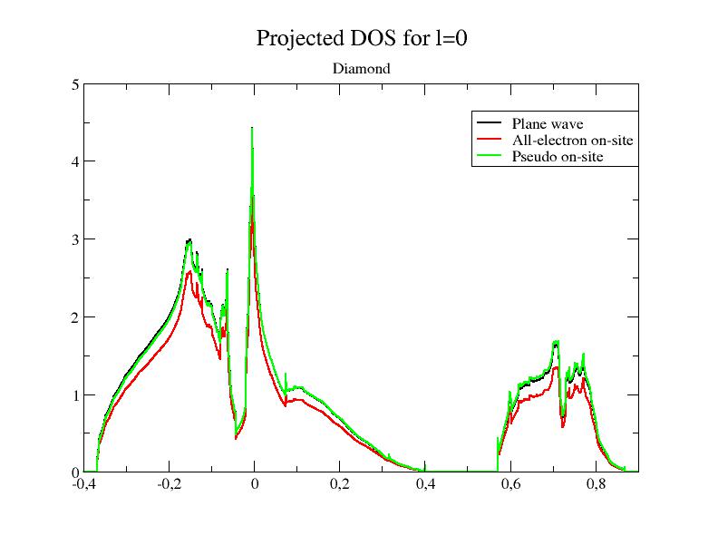
Note that, in the previous section, we used a "standard" PAW
dataset,
with 2 partial waves per angular momentum. It is generally the best
compromise between the completeness of the partial wave basis and the
efficiency of the PAW dataset (the more partial waves you have, the
longer the CPU time used by ABINIT is).
Let's have a look at the
~abinit/tests/Psps_for_tests/6c.lda.atompaw file. The
sixth line indicates the number of partial waves and their l angular momentum.
In the present file, "0 0 1 1" means "two
l=0 partial waves, two l=1
partial waves".
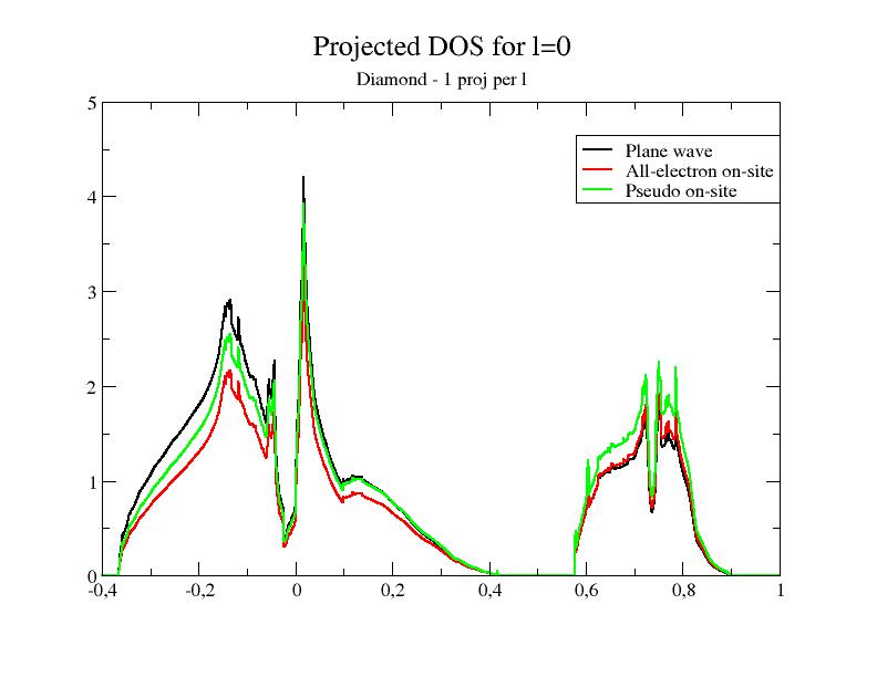
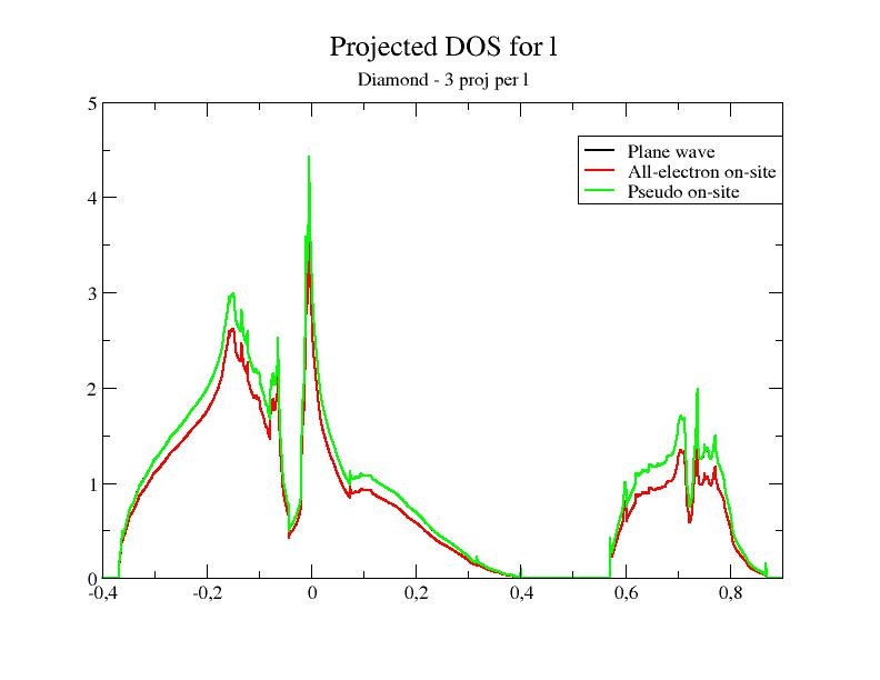
Now, let's open the
~abinit/tests/Psps_for_tests/6c.lda.test-2proj.atompaw and
~abinit/tests/Psps_for_tests/6c.lda.test-6proj.atompaw
files. In the first file, only one partial wave per l is present; in
the second one, 3 partial waves per l
are present. In
other words, the completeness of the partial wave basis increases when
you use 6c.lda.test-2proj.atompaw,
6c.lda.atompaw and 6c.lda.test-6proj.atompaw.
Now, let's plot the DOS for the two new PAW datasets.
As usual, the validity of a "pseudopotential" (PAW dataset) has to
be
checked by comparison, on known structures, with known results. In the
case of diamond,
lots of computations and experimental results exist.
Very important remark: the validity (completeness
of plane wave basis and partial wave basis) of PAW calculations
should always
be checked by comparison with all-electrons computation results (or
with other existing
PAW results); it should not be done by comparison with experimental
results.
As the PAW method has the same accuracy than all-electron methods,
results should be very close.
Concerning diamond,
all-electron results can be found (for instance) in PRB 55, 2005 (1997).
With the famous WIEN2K
code (which uses the FP-LAPW
method), all-electron equilibrium parameters for diamond (for LDA) are:
abinit < tpaw1_5.files > tmp-log
From
the tpaw1_5.out
file, you can extract the 7 values of acell
and 7 values
of etotal,
then put them into a file and plot it with a graphical tool. You should
get: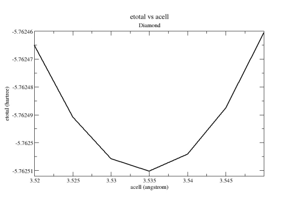
8.a Mixing scheme for the Self-Consistent cycle; decomposition of the total energy.
The use of an efficient mixing scheme in the self-consistent loop is a crucial point to minimize the number of steps to achieve convergence. This mixing can be done on the potential or on the valence density. By default, in a norm-conserving pseudopotential calculation, the mixing is done on the potential; but, for technical reasons, this choice is not optimal for PAW calculations. Thus, by default, the mixing is done on the density when PAW is activated.8.b Overlap of PAW spheres
In
principle, the PAW formalism is only valid for non-overlapping
augmentation
regions (PAW spheres). But, in usual cases, a small overlap between
spheres is acceptable.
By
default, ABINIT checks that the distances between atoms are large
enough to avoid overlap; a "small" voluminal overlap of 5% is accepted
by default. This value can be tuned with the pawovlp input keyword. The overlap
check can even be by-passed with pawovlp=-1.
Important warning: while a small overlap can be acceptable for the augmentation regions, an overlap of the compensation charge densities has to be avoided. The compensation charge density is defined by a radius (named rshape in the PAW dataset file) and an analytical shape function. The overlap related to the compensation charge radius is checked by ABINIT and a WARNING is eventually printed...
Also note that you can control the compensation charge radius and shape function while generating the PAW dataset (see tutorial PAW2).
8.c Printing volume for PAW
If you want to get more detailed output concerning the PAW computation, you can use the pawprtvol input keyword. See its description in the user's manual...8.d Additional PAW input variables
Looking at the [[varset:basic|~abinit/doc/input_variables/varset_basic.html]] file, you can find input ABINIT keywords specific to PAW. They are to be used when tuning the computation, in order to gain accuracy or save CPU time.The above list is not exhaustive. several other keywords can be used to tune ABINIT PAW calculations.
8.e PAW+U
If the system under study contains strongly correlated electrons, the LDA+U method can be useful. It is controlled by the usepawu, lpawu, upawu and jpawu input keywords. Note that the formalism implemented in ABINIT is approximate, i.e. it is only valid if: