ABINIT: the tutorial
The lessons of this tutorial are aimed at teaching the use of ABINIT, in the
UNIX/Linux OS and its variants (Mac OS X, AIX ...). They might be used
for other operating systems, but the commands have to be adapted.
Note that they can be accessed from the ABINIT web site as well as
from your local ~abinit/doc/tutorial/welcome.html file. The latter
solution is of course preferable, as the response time will not depend
on the network traffic.
Copyright (C) 2000-2017 ABINIT group (XG,RC)
This file is distributed under the terms of the GNU General Public License, see
~abinit/COPYING or
http://www.gnu.org/copyleft/gpl.txt .
For the initials of contributors, see ~abinit/doc/developers/contributors.txt .
At present, more than thirty lessons are available. Each of them is
at most two hours of student work. Lessons 1-4 cover the basics, other
lectures are more specialized.
Before following the tutorials, you should have read the "new user's guide", as well as
the pages 1045-1058 of the paper "Iterative minimization
techniques for ab initio total-energy calculations: molecular dynamics
and conjugate gradients", by M.C. Payne, M.P. Teter, D.C.
Allan, T.A. Arias and J.D. Joannopoulos, Rev. Mod. Phys. 64, 1045
(1992) or, if you have more time, you should browse through the
Chaps. 1 to 13 , and appendices L and M of the book Electronic
Structure. Basic Theory and Practical Methods. R. M. Martin. Cambridge
University Press (2004) ISBN 0 521 78285 6. The latter reference
is a must if you have not yet used another electronic structure code or
a Quantum Chemistry package.
After the tutorial, you might find it useful to learn about the test
cases contained in the subdirectories of ~abinit/tests/, e.g. the
directories fast, v1, v2, ... v6, that provide many example input files.
You should have a look at the README files of these directories.
Additional information can be found in the ~abinit/doc directory,
including the description of the ABINIT project, guide lines for
developpers, more on the use of the code (tuning) ...
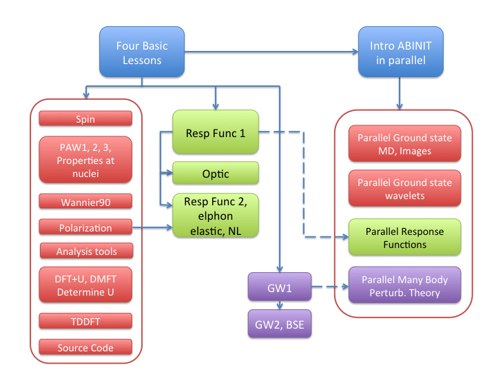
Some lessons depends on other lessons. The following schema should
help you to understand these dependencies. In blue, one has the basic lessons. The blocks in red
represents additional lessons related to ground-state features of ABINIT. Response-function
features of ABINIT are explained in the lessons in the green blocks. Finally,
the Many-Body Perturbation Theory capabilities are demonstrated in the lessons belonging to the violet blocks.
The right-hand side blocks gather the lessons related to the parallelism inside ABINIT.
Brief description of each lesson's content
The lessons 1-4 present the basic concepts, and form a global
entity: you should not skip any of these.
- The lesson 1 deals with the H2
molecule : get the total energy, the electronic energies, the charge
density, the bond length, the atomisation energy
- The lesson 2 deals again with the H2
molecule: convergence studies, LDA versus GGA
- The lesson 3 deals with crystalline
silicon (an insulator): the definition of a k-point grid, the smearing
of the cut-off energy, the computation of a band structure, and again,
convergence studies ...
- The lesson 4 deals with crystalline
aluminum (a metal), and its surface: occupation numbers, smearing the
Fermi-Dirac distribution, the surface energy, and again, convergence
studies ...
Other lessons present more specialized topics.
There is a group of lessons that can be started without any other prerequisite than the lessons 1 to 4, and that you can do in any order (there are some exceptions, though):
- The lesson on spin in ABINIT
presents the properties related to spin: spin-polarized calculations
and spin-orbit coupling.
- The lesson on the use of PAW (PAW1)
presents the Projector-Augmented Wave method, implemented in ABINIT as
an alternative to norm-conserving pseudopotentials, with a sizeable
accuracy and CPU time advantage.
- The lesson on the generation of PAW
atomic data files (PAW2) presents the generation of atomic data
for use with the PAW method. Prerequisite : PAW1.
- The lesson on the validation of a PAW
atomic datafile (PAW3) demonstrates how to test a generated PAW
dataset using ABINIT, against the ELK all-electron code, for diamond
and magnesium. Prerequisite : PAW1 and PAW2.
- The lesson on the properties of the nuclei
shows how to compute the electric field gradient. Prerequisite : PAW1.
- The lesson on Wannier90 deals
with the Wannier90 library to obtain Maximally Localized Wannier
Functions.
- The lesson on polarization and finite
electric field deals with the computation of the polarization of
an insulator (e.g. ferroelectric, or dielectric material) thanks to
the Berry phase approach, and also presents the computation of
materials properties in the presence of a finite electric field (also
thanks to the Berry phase approach).
- The lesson on Analysis
Tools deals with the use of the CUT3D utility to analyse
wavefunctions and densities.
- The lesson on DFT+U shows
how to perform a DFT+U calculation using ABINIT, and will lead to
compute the projected DOS of NiO. Prerequisite : PAW1.
- The lesson on DFT+DMFT shows
how to perform a DFT+DMFT calculation on SrVO3 using projected Wannier functions. Prerequisite : DFT+U.
- The lesson on the calculation of effective interactions U and J by the cRPA method shows how to determine the U value with the constrained Random Phase Approximation using projected Wannier orbitals. Prerequisite : DFT+U.
- The lesson on the determination of U
for DFT+U shows how to determine the U value with the linear response method, to be used in the
DFT+U approach. Prerequisite : DFT+U.
- The lesson on TDDFT deals with the
computation of the excitation spectrum of finite systems, thanks to
the Time-Dependent Density Functional Theory approach, in the
Cassida formalism.
- The lesson "Source code"
introduces the user to the development of new functionalities in
ABINIT: in this lesson, one learns how to add a new input variable
...
There is an additional group of lessons on response functions
(phonons, optics, dielectric constant, electron-phonon interaction,
elastic response, non-linear optics, Raman coefficients,
piezoelectricity ...), for which some common additional information are
needed:
- The lesson Response-Function 1 (RF1)
presents the basics of response-functions within ABINIT. The example
given is the study of dynamical and dielectric properties of AlAs (an
insulator): phonons at Gamma, dielectric constant, Born effective
charges, LO-TO splitting, phonons in the whole Brillouin zone. The
creation of the "Derivative Data Base" (DDB) is presented.
- The lesson Response-Function 2 (RF2)
presents the analysis of the DDBs that have been introduced in the
preceeding lesson RF1. The computation of the interatomic forces and
the computation of thermodynamical properties is an outcome of this
lesson.
- The additional information given by lesson RF1 opens the door to
The lesson on Optic, the utility that
allows to obtain the frequency dependent linear optical dielectric
function and the frequency dependent second order nonlinear optical
susceptibility, in the simple "Sum-Over-State" approximation.
- The additional information given by lesson RF1 and RF2 opens
the door to a group of lessons that can be followed independently of
each other: The lesson on the
electron-phonon interaction presents the use of the utility MRGKK
and ANADDB to examine the electron-phonon interaction and the
subsequent calculation of superconductivity temperature (for bulk
systems).
- The lesson on the elastic
properties presents the computation with respect to the strain
perturbation and its responses: elastic constants,
piezoelectricity.
- The lesson on static non-linear
properties presents the computation of responses beyond the linear
order, within Density-Functional Perturbation Theory (beyond the
simple Sum-Over-State approximation): Raman scattering efficiencies
(non-resonant case), non-linear electronic susceptibility,
electro-optic effect. Comparison with the finite field technique
(combining the computation of linear response functions with finite
difference calculations), is also provided.
An additional lesson has been developed outside the standard structure of the ABINIT tutorial,
in the experimental Wiki of ABINIT,
the lesson on temperature dependence of the electronic structure.
There is another additional group of lessons on many-body
perturbation theory (GW approximation, Bethe-Salpeter equation),
to be done sequentially):
The first lesson on GW (GW1) deals with
the computation of the quasi-particle band gap of Silicon
(semiconductor), in the GW approximation (much better than the
Kohn-Sham LDA band structure), with a plasmon-pole model.
The second lesson on GW (GW2) deals with
the computation of the quasi-particle band structure of Aluminum, in
the GW approximation (so, much better than the Kohn-Sham LDA band
structure) without using the plasmon-pole model.
The lesson on the Bethe-Salpeter Equation (BSE) deals with the
computation of the macroscopic dielectric function of Silicon within
the Bethe-Salpeter equation.
Concerning parallelism, there is another set of specialized
lessons. For each of these lessons, you are supposed to be familiarized
with the corresponding tutorial for the sequential calculation.
- An introduction on ABINIT in
Parallel should be read before going to the next lessons about
parallelism. One simple example of parallelism in ABINIT will be
shown.
- Parallelism for ground-state
calculations, with plane waves presents the combined k-point (K),
plane-wave (G), band (B), spin/spinor parallelism of ABINIT (so, the
"KGB" parallelism), for the computation of total energy, density, and
ground state properties
- Parallelism for molecular
dynamics calculations
- Parallelism based on "images",
e.g. for the determination of transitions paths (string method),
that can be activated on top of the "KGB" parallelism for force
calculations.
- Parallelism for ground-state
calculations, with wavelets presents the parallelism of ABINIT,
when wavelets are used as a basis function instead of planewaves, for
the computation of total energy, density, and ground state properties
- Parallelism of response-function
calculations - you need to be familiarized with the calculation of
linear-response properties within ABINIT, see the tutorial Response-Function 1 (RF1)
- Parallelism of Many-Body
Perturbation calculations (GW) allows to speed up the calculation of
accurate electronic structures (quasi-particle band structure,
including many-body effects).
The following topics should be covered later:
- the choice of pseudopotentials
NOTE that not all features of ABINIT are covered by these
tutorials. For a complete feature list, please see the
~abinit/doc/features/ directory. For examples on how to use these
features, please see the ~abinit/tests/* directories and their
accompanying README files.
Copyright (C) 2000-2017 ABINIT group (XG,RC)
This file is distributed under the terms of the GNU General Public License, see
~abinit/COPYING or
http://www.gnu.org/copyleft/gpl.txt .
For the initials of contributors, see ~abinit/doc/developers/contributors.txt .